Part 2 Extra: More Formatting for your Excel Runescape Hiscores Tracker

It's great to learn that so many people are using this guide to make their own Runescape Hiscores Tracker in Microsoft Office Excel! Glad to have you along for the ride. *blows kisses*

Some people have been asking me questions. They're doing it in-game or on Sal's Realm of Runescape, just about everywhere but here, where the answers might be useful for everyone else. Nevertheless, I will answer them here.

How Do You Get Rid of the Gridlines in the Background of an Excel Worksheet?

This one is very easy. It will take about a second to do it.

• Select the 'View' tab from the top Excel toolbar.
• Click the box next to 'Gridlines'.

That's it! Though remember that you did that, if you find it easier to work with the gridlines when you're next creating things. Just tick the box again to put them back.

How Do You Add Gridlines/Cell Borders Inside the Table?

This is done in the same way that we added the outer border. It's simply another option within that pull down menu.

• Highlight your table.
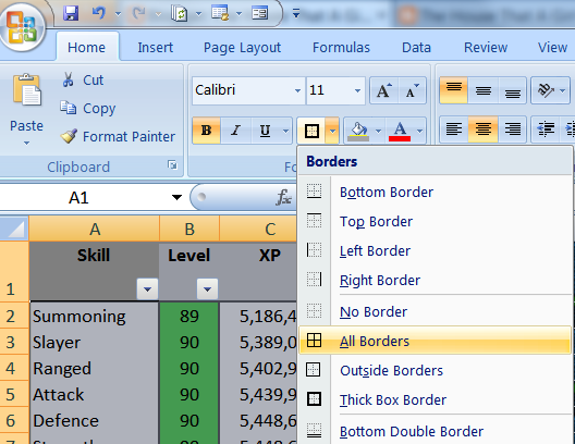
• Click on the borders button, in the 'font' category of the 'Home' tab.
• Select 'All Borders' from the pull down menu and click it.

NB This will remove your thick outer borders, if you had those added. Just reinstate them in the same way that you did it originally.

How Do You Move Your Averages Hiscores Chart?

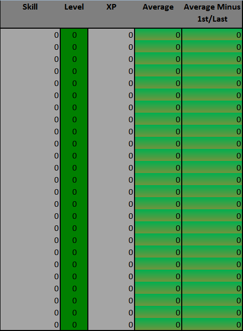
I guided you through creating this table in the first five columns of your worksheet, but it is possible to copy and paste it elsewhere. You just need to do a small amount of adjusting once it's there.

• Highight all five columns by clicking on A and dragging your mouse to E.
• Right-click anywhere in the highlighted columns.
• Chose 'copy' from the pull-down menu.
• Right-click on the first cell of the area you want to display it.
• Select 'paste special' from the pull-down menu.

This will produce a table with all of the colouring and formatting, but no data. Don't fret about this. The formulas are all still there, but those in the first three columns are pointing to the wrong place. The act of moving them means that Excel automatically adjusts them, which is sometimes great and sometimes not.

• Click on the first cell in the 'Skill' column.
• Paste in this formula: =Data!B2
• Click on the little square to drag that formula down to the bottom of the table.
• Click on the first cell in the 'Level' column.
• Paste in this formula: =Data!C2 and drag that down too.
• Click on the first cell in the 'XP' column.
• Paste in this formula: =Data!F2 and drag that down too.

All good! Please note that if you called your data worksheet something else, you need to swap 'Data' in those formulas to the name you called it.

A simple alternative method is to insert columns or rows before your table.

• Highlight the A column.
• Right-click anywhere in the highlighted section.
• Select 'insert' from the pull-down menu.

You just need to repeat that until the table is where you want it to be.

If anyone has any more questions, just comment and I'll do my best to answer them for you.